Arrays, Statistics and Polynomials

Introduction

This week, we will continue to work with arrays and plots. We have already seen how to generate and plot arrays. Now, we will learn additional ways of accessing the contents of an array by, for example, getting the largest and smallest entries. We will also learn how to extract basic statistical information from arrays and to plot histograms. We will demonstrate this by generating and analyzing a series of random numbers.

Also, we will introduce functions to generate, plot, integrate and differentiate polynomials. We will also learn how to fit polynomials to data.

Useful Links

• Array sorting and searching
• Histogram demo code
• Polynomials

Syntax Summary

Manipulating /Analyzing Arrays (For a 1D array x)

All of these functions are contained in the NumPy package.

Function		Syntax
Length of an array		len (a)
Extract an entry from an array Remember that the entries of an array of length n are numbered from 0 to n-1.	Return entry 0	a[0]
	Return entry 4	a[4]
	Return the last entry	a[-1]
	Return the second to last entry	a[-2]
Return part of a 1D array a	return entries r to (s - 1)	a[r:s]
	return entries r to end	a[r:]
	return entries start to (s - 1)	a[:s]
	return entries s to q from end	a[s:-q]
	return entries r to (s-1) with a step of t	a[r:s:t]
Maximum and minimum	return the maximum entry	max(a)
	return the position (argument) of maximum entry	argmax(a)
	return the minimum entry	min(a)
	return the position (argument) of minimum entry	argmin(a)
Sort array in ascending order		sort(a)
Sum the entries in an array		sum(a)
Basic statistics	calculate the mean of the entries	mean(a)
	calculate the median of the entries	median(a)
	calculate the variance of the entries	var(a)
	calculate the standard deviation of the entries	std(a)
Truth testing	identify entries of a that are smaller than x (returns array of True/False)	a<x
	return all entries of a that are less than x	a[a<x]
	return all entries of b that correspond to entries of a < x (only works is a, b are same size)	b[a<x]

Histograms

Histograms are contained in the Matplotlib package.

Function	Syntax
Make a histogram of data r	hist(r)
Histogram with specific number of bins	hist(r, bins=20)
Histogram data over a given range	hist(r, range=(0.1)
Histogram with y-axis on a log scale	hist(r, log=True)
Histogram with given transparency	hist(r, alpha=0.4)

Polynomials

Polynomials are part of the NumPy package.

Function	Syntax
Generate a polynomial p(x) = ax2 + bx + c	p = poly1d([a, b, c])
Evaluate a polynomial, p, at an array of points x	p(x)
Calculate the roots of a polynomial p	roots(p)
Calculate the coefficients of a polynomial from its roots (x-q)(x-r)(x-s)	poly([q, r, s])
Generate a polynomial with roots q, r, s	p = poly1d(poly([q,r,s]))
Differentiate a polynomial)	polyder(p)
Integrate a polynomial	polyint(p)
Find coefficients of a best fit polynomial of degree n to data arrays x and y	polyfit(x, y, n)

Worksheet

Accessing the contents of an arrays

In this section, we will learn more about accessing entries of arrays. We will start with the most basic methods, before moving on to some more complex operations and also basic statistics.

Accessing array entries

To get started, let's create a very basic array

a = arange(10)
print(a)

You will see that a contains ten entries: the integers from 0 to 9. You could have generated the same array by requesting

a = arange(0,10,1)

i.e. an array that goes from 0 to 10 in steps of 1 and does not include the final value. When we just use arange(10), the function assumes that we wish to start at zero and have a step size of 1. Next, we will run through various ways of examining the contents of the array and accessing various entries of the array.

1. You already know how to print out the contents of the array, by typing

print(a)

2. The length of an array (the number of elements in the array) is given by the function len as

len(a)

3. The entries in the array are numbered, and if you want to know the value of a given entry in the array you can just ask for it. Note that in python the entries are numbered starting at zero. So, what you might consider the first entry of the array is actually entry zero. This is quite standard in computing. In an array of length n, the entries are numbered (0, 1, 2, ..., n-1).
   You can access any entry of the array that you like. For example,

   x = a[0]
   print(x)

   will generate a new variable, x, which contains entry zero of the array a. Since the example array is an array of integers, the variable x will be an integer. If a was an array of floats, then x would be a float.

   print(a[3])
   

   returns entry three. We have deliberately set up our array a so that the entry zero is equal to zero, etc.
   If you try to access an entry that doesn't exist -- for example, entry 10 in an array of length 10 -- then you get an error

   print(a[10])
   

   gives the error IndexError: index out of bounds.
4. You can access entries by counting backwards from the end, for example:

   print(a[-1])
   

   prints the last entry.

   print(a[-2])
   

   prints the second to last entry.
5. You can access a range of entries in the array by specifying the range that you are interested in. For example

   b = a[3:8]
   

   will create an array b which contains entries 3 to 7 from array a (remember that we start counting at zero). Note that it does not include entry 8! This is similar to arange where the returned array includes the min value but not the max.
   As a default, if you leave out first number, then it's assumed that you want to start at the start of the array. Similarly, leaving out the second number will, by default, continue to the end. So

   b = a[3:]
   

   will return entry 3 to the end,

   b = a[:8]
   

   will return up to (but not including) entry 8. Specifying neither number will return the entire array. So, you should find that

   print(a)
   print(a[:])

   both return the same thing.
6. This syntax can also be used to access every second or third (or Nth) item in an array, using the form

   a[start:stop:step]
   

   Again, notice that the syntax is very similar to what we have seen before with arange. For example, since every other entry is even, we could extract the even numbers from the array a using:

   even = a[0:10:2]
   

   In this example we are covering the whole length of the array, so you can miss out the start and/or stop numbers to run from the first to last entry:

   even = a[::2]
   

Basic Statistics

As well as asking for entries based on their position, we can also ask for the largest and smallest entries in the array. Last week we learned several ways of creating arrays (using linspace, logspace, zeros, ones, ...). To illustrate finding maximum and minimum, we will make use of an array of random numbers. To generate an array of random numbers, with values between zero and 1, type:

r = rand(100)
print(r)

This has generated an array containing 100 random numbers that are uniformly distributed between zero and one. Now, let's investigate in a bit more detail the entries in the array. You can use the commands above to access specific entries in the array. There are a number of other things that you can easily calculate.

1. First, we might want to know what the largest number of the 100 is. You could scan through the numbers and find it, but it's much easier to do

   max(r)
   

   We may also be interested in where in the array the largest entry is. This is given by

   argmax(r)
   

   You can check that this is all consistent by retrieving the entry at that position

   r[argmax(r)]
   

   and checking that the value agrees with max(r). Exactly the same thing can be done with the smallest entry in the array, accessed using

   min(r)
   argmin(r)

2. You can sort an array in increasing order.

   s = sort(r)
   

   Having done that, it should be easy to verify that the max and min that you obtained above are correct as the min will be the zeroth entry and the max will be the last entry.
3. You can find the average entry of the array. There are two averages available, the mean and median:

   mean(r)
   median(r)

   The mean is the sum of all the entries divided by the number of entries. Check that this is true by calculating the sum divided by the length of the array.
   The median corresponds to the middle value in the array. Since there are 100 entries in this array, it will be the value half way between the entry 49 and entry 50 of the sorted array. Verify this.
4. You can also calculate the variance and standard deviation of the values in the array using

   std(r)
   var(r)

   For a uniform distribution with values between zero and 1, the standard deviation is 1/√12. The standard deviation of the points in the array r should be close to this, but not exactly equal as we have only sampled 100 points from the distribution.

Truth testing on Arrays

The inequalities introduced in Week 1 can be used to test the values in an array, returning a boolean (True/False) array that shows which values satisfy the inequality. For example, we can use them to find out which of the random numbers in the array r are greater than 0.5:

print(r>0.5)

This gives an array of the same size as r where each entry is either True (if the corresponding entry in r is greater than 0.5) or False (if not). If you do the same thing on the sorted array s then you should get a bunch of False entries followed by a bunch of True entries.

To work out how many entries in r are greater than 0.5, we simply sum over the array of True/False. Each True counts as 1 and each False as 0. So

sum(r>0.5)

gives a count of the number of entries larger than 0.5. If we are interested in the values of those entries, we can make a new array containing only the entries of r which are greater than 0.5 as

r_big = r[r>0.5]

Note: You can also use this to return the values in a different array of the same length that correspond to those for which r>0.5. For example

a = arange(100)
a_big = a[r>0.5]

Histograms

Histograms are a very useful way to graphically display 1D data. You can plot a histogram for an array r using hist(r), for example:

r = rand(1000)
hist(r)

Specifying bins

The type of histogram you plot is set automatically as having 10 bins evenly spaced over the range of the data and plotted on a linear scale. You can change this for plotting different kinds of data. For example:

hist( r, bins=20 )

will plot a histogram with 20 bins instead on 10.

It is often convenient to fix the minimum and maximum values of the bins. To do this, you need to specify the range that the histogram should cover

hist(r, range=(0,1), bins=20)

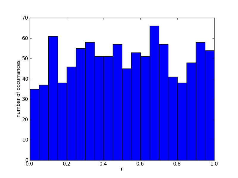
Figure 1: A histogram of 1,000 random numbers distributed between 0 and 1 plotted using 20 bins

Log scale

You can also plot a histogram on the a log scale using

hist( r, log=True )

will plot the histogram with the y axis on a log scale.

Multiple histograms with transparency

When plotting several histograms on one graph to compare them, it is often difficult to distinguish the shapes because they overlap each other. The following code can be used to make the plots slightly transparent so that the shapes of the plots behind can still be seen:

hist(r, alpha=0.4)

Alpha is a coefficient representing the level of transparency and can take any value between 0 and 1.

Polynomials

NumPy has a set of functions for generating, evaluating, differentiating, integrating and fitting polynomials. The are described on the Poly1d page.

Generating a polynomial from coefficients

The poly1d() function can be used to define polynomials. To use it, you need to specify the coefficients of the polynomial. For example

p = poly1d([2, 3, 4]) 
print(p)

If you enter this code you will see that this makes a polynomial with the equation 2x²+3x+4, i.e. highest order term first. The number of terms defines the degree of the polynomial. Take care when entering polynomials containing coefficients that are zero. For example 2x³ +5x must be entered with coefficients [2, 0, 5, 0].

Create a plot of a polynomial

This requires four steps:

• Define the polynomial
• Generate an array of x points for the range of the polynomial of interest
• Evaluate the polynomial at each point of the x array
• Plot the function

Define the polynomial p= 4x² + 3x - 10

p=poly1d([4,3,-10])

Create an x array between -5 and 5

x=linspace(-5, 5, 100)

Create a second array by evaluating the polynomial for each point in the x array

y = p(x)

Plot x against y

plot(x,y)
grid()
#or alternatively
plot(x,p(x))
grid()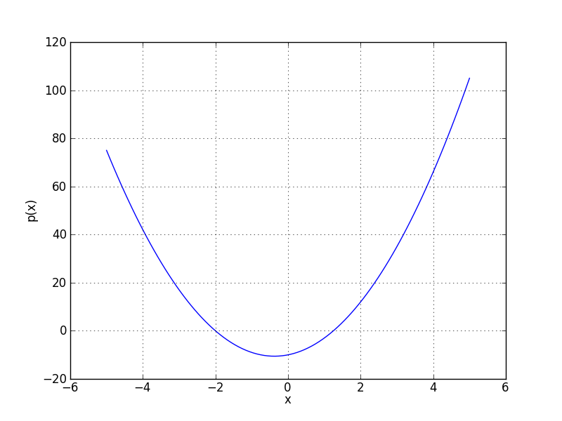

Figure 3: A plot of the polynomial function p = 4x² + 3x - 10 as generated by the code above

The roots of a polynomial

The solutions of the equation p(x) = 0 are called the roots of a polynomial p. Written in the form (x-q)(x-r)=0, q and r are the roots. An nth order polynomial has n roots. Wherever the polynomial crosses the x axis, it has a real root. If it touches the x axis, it has two (or more) coincident real roots. If an n-th order polynomial has fewer than n real roots, the remaining roots are complex.

To find the roots of the polynomial p that we defined above, type

roots(p)

In this example you should get an array of two real roots, - 2 and 1.25 (in agreement with expectations from figure 3).

Generate a polynomial from its roots

The poly() function is the reverse of the roots() function. It calculates the coefficients of a polynomial from a given sequence of roots. Try the following

poly([-2,1.25])

This should return “array([ 1. , 0.75, -2.5 ])” containing the coefficients of the polynomial. This does not agree with the original polynomial p = 4x² + 3x - 10. The reason is that the roots of a polynomial determine the polynomial up to an overall scaling. By default, the coefficients returned are normalised so that the first coefficient (coefficient of the highest order) is 1.

To demonstrate this, use the code below to add a plot of the polynomial produced using the roots of the last problem. Note that the poly function does not return a polynomial! It returns a list of values that can be used to make a polynomial using the poly1d function.

q=poly1d(poly([-2,1.25]))
plot(x,q(x))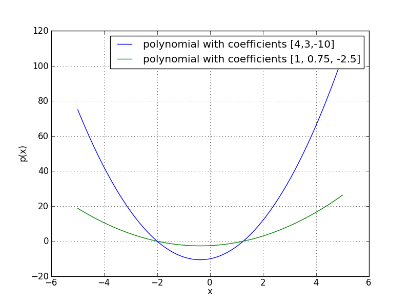

Figure 4: A plot of the polynomial functions p = 4x² + 3x - 10 and r = x² + 0.75x - 2.5, as generated by the code in this section.

Differentiating and integrating polynomials

There are routines in NumPy to integrate and differentiate polynomials. As an example, suppose you wanted to find the minimum of the polynomial p plotted in figure 3. You could do that by

• defining the polynomial
• differentiating it
• finding the roots of the differentiated polynomial

In code that is

p=poly1d([4,3,-10])
dp_dx = polyder(p)
roots(dp_dx)

That will give the result of -0.375, which certainly looks right from figure 3 (and can be verified by doing the calculation by hand).

Fitting polynomials to data

There is a function which will fit a best fit polynomial to a set of data. In future weeks, we will use this to generate best fit lines through experimental data. Here, as an example, we will consider fitting a polynomial to a sine curve. First, generate the data

x = linspace(-pi, pi, 100)
y = sin(x)
plot(x, y, label="sin(x)" )

Then, can fit a first order polynomial (a straight line) to the sine curve between -π and π using

c1 = polyfit(x, y, 1)
p1 = poly1d(c1)

Note: polyfit returns the coefficients of the polynomial and we must use poly1d to obtain the polynomial itself. Then, plot the best fit straight line

plot(x, p1(x), label="1st order polynomial fit" )

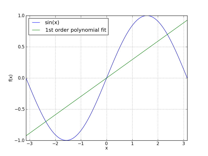
Figure 5: A sine curve plotted between -π and π and a first order polynomial fit to the data over the same range.

Excercises